Perceptron Blog

Perceptron source code: click here

Let’s begin by replicating the example from class: making two sets of points and running the perceptron algorithm on them

import numpy as np
import pandas as pd
import seaborn as sns
from matplotlib import pyplot as plt
from sklearn.datasets import make_blobs
from perceptron import Perceptron
import numpy as np
import pandas as pd
import seaborn as sns
from matplotlib import pyplot as plt

np.random.seed(12345)

n = 100
p_features = 3

X, y = make_blobs(n_samples = 100, n_features = p_features - 1, centers = [(-1.7, -1.7), (1.7, 1.7)])

p = Perceptron()
p.fit(X, y,1000)

def draw_line(w, x_min, x_max,pos,**kwargs): # "pos" = position, i.e. where to plot (plt, ax)
  x = np.linspace(x_min, x_max, 101)
  y = -(w[0]*x + w[2])/w[1]
  pos.plot(x, y, color = "black", linestyle = "dashed" if kwargs else "solid")

fig = plt.scatter(X[:,0], X[:,1], c = y)
fig = draw_line(p.w, -2, 2,plt)

xlab = plt.xlabel("Feature 1")
ylab = plt.ylabel("Feature 2")

This perceptron works! We can show that it converges by showing the change in accuracy - how many points are correctly classified - over time.

fig = plt.plot(p.history)
xlab = plt.xlabel("Iteration")
ylab = plt.ylabel("Accuracy")

p.score(X, (2*y-1))

1.0

How does the perceptron algorithm work?

The key part of the perceptron algorithm is the update step. In my code, this is done in both the fit and update methods.

Mathematically, this can be represented as: (on a personal note this is the first thing I have ever done in LaTeX and I’m really proud of it)

\(\hat{w}^{(t+1)} = \hat{w}^t + \mathbb{1}(\tilde{y}_i(\vec{\hat{w}^t} \cdot \vec{\tilde{x}_1}) <0){\tilde{y}_i} {\tilde{x}_1}\)

Within the fit() method, this is done in the following code:

y_hat = np.dot(w,X_i)
w_i = ( (np.multiply(y_hat, y_i) >= 0) * w_i)  + ( (np.multiply(y_hat, y_i) < 0) * (w_i + np.multiply(y_i,X_i)) )

The logic is actually fairly simple. Y_hat represents the predicted score for X_i, the current index/value being considered. If y_hat is correctly classified, multiplying it by y_i should yield True, equal to 1 in Python. The other part of the equation checks to see if this product is less than 1 (using 1s and -1s instead of 1s and 0s for our y values makes this possible). If it is, this expression will evaluate to True, which is equal to 1 in Python.

Only one of these expressions is true at any given time. When False, these evaluate to zero.

If the first expression is True, aka when it is equivalent to 1, it preserves the current weight vector, while the second expression, equal to zero, nullifies its coefficient.

When the second expression is True and therefore equal to 1, it is multiplied by the sum of w_i (the current weight vector) and the product of the feature matrix (X) at index i, and the classification matrix (y) at index i. This sounds complicated, but really this line of code is just either keeping the old weight vector if it classified point i correctly, or adding or subtracting the value it incorrectly classified to ensure that it classifies it correctly in the next iteration.

This logic is the same in the update method. The only difference is that update accepts a weight vector as a parameter, running only a single step of the Perceptron algorithm rather than to completion.

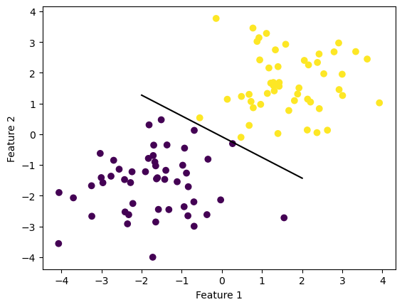
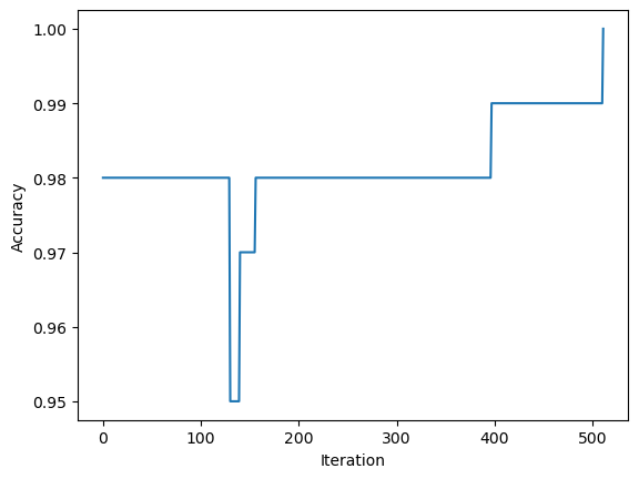
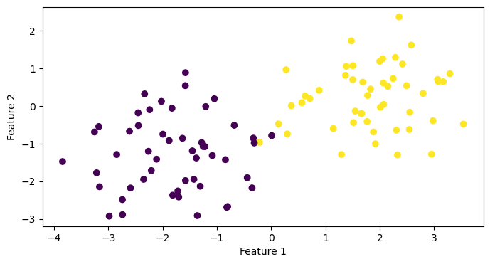
If the data are linearly separable, then the perceptron algorithm will converge.

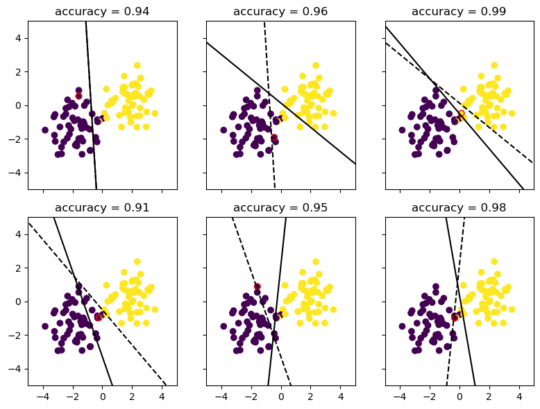
Let’s vizualise the process of improvement by showing the progression of the Perceptron algorithm over time.

fig = plt.scatter(X[:,0], X[:,1], c = y)
xlab = plt.xlabel("Feature 1")
ylab = plt.ylabel("Feature 2")
p2 = Perceptron()

Let’s see how the algorithm updates over time…

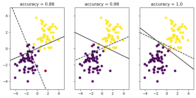
These three plots only show instances where the weight vector updates (that is to say, when the algorithm misclassifies a point and updates the weight vector to reflect this). This ensures that we actually see how the Perceptron algorithm corrects itself over time. Otherwise, we might just see three cases where it correctly classifies a point and nothing changes. BORING!!!

w_next = np.random.rand(p_features)

plt.rcParams["figure.figsize"] = (8, 4)
fig, axarr = plt.subplots(1, 3, sharex = True, sharey = True)
X_1 = np.append(X, np.ones((X.shape[0], 1)), 1)
score_prev = 0

for ax in axarr.ravel():
    ax.set(xlim = (-5, 5), ylim = (-5, 5))
    w_prev = w_next
    ax.scatter(X[:,0],X[:,1], c = y)
    draw_line(w_prev, -10, 10,ax,linestyle = "dashed") 
    done = False
    while done == False:
        w_next, score, i = p2.update(X,y,w_prev)
        if (score_prev != score) or score == 1 :
            done = True
    score_prev = score
    draw_line(w_next, -10, 10,ax)
    ax.scatter(X[i, 0], X[i, 1],color = "none", facecolors = "none", edgecolors = "red")
    accuracy = (score)
    ax.set_title(f"accuracy = {accuracy}")
    
plt.tight_layout()

It is fairly easy to see that the algorithm updates when it missclassifies a point, gradually improving until it achieves convergence.

What if the data are not linearly separable?

Let’s repeat the same experiment as above, only this time, using two clouds of points that are NOT linearly separable.

We can achieve this easily with the make_blobs function by making the centers closer to one another.

X2, y2 = make_blobs(n_samples = 100, n_features = p_features - 1, centers = [(-1.7, -1.3), (1.7,0.3)])

fig = plt.scatter(X2[:,0], X2[:,1], c = y2)
xlab = plt.xlabel("Feature 1")
ylab = plt.ylabel("Feature 2")

plt.rcParams["figure.figsize"] = (8, 6)
fig1, axarr1 = plt.subplots(2, 3, sharex = True, sharey = True)

w_next1 = np.random.rand(p_features)

score_1 = 0

for ax in axarr1.ravel():
    ax.set(xlim = (-5, 5), ylim = (-5, 5))
    w_prev1 = w_next1
    ax.scatter(X2[:,0],X2[:,1], c = y2)
    draw_line(w_prev1, -10, 10,ax,linestyle = "dashed") 
    done = False
    while done == False:
        score_prev = score1
        w_next1,score1,i = p2.update(X2,y2,w_prev1)
        if (score_prev != score1) or score1 == 1 :
            done = True
    draw_line(w_next1, -10, 10,ax)
    ax.scatter(X2[i, 0], X2[i, 1],color = "none", facecolors = "none", edgecolors = "red")
    accuracy = (score1)
    ax.set_title(f"accuracy = {accuracy}")
    
plt.tight_layout()

We can see that the algorithm still updates and tries to correct itself, but is unable to achieve 100% accuracy. Including more subplots helps to show that this process of guessing but never achieving convergence will continue infinitely.

Can Perceptron work in more than 2 dimensions?

Only one way to find out…

Let’s start by generating a 5D feature matrix.

X5d = np.random.rand(100,5)
y5d = np.random.choice([0, 1], size=100)

We now have a random 5d feature matrix, and a random binary classification for each point.

Let’s try to run it with 10,000 max steps…

p3 = Perceptron()

p3.fit(X5d,y5d, max_steps = 10000)

Did it work?

p3.score(X5d,2*y5d-1)

0.6

It works! It makes sense that it wouldn’t achieve convergence on a completely random set of points and classifications.

It is worth asking, though, is it theoretically possible to have a linearly separable set of points in 5 (or more) dimensions?

It is pretty straightforward to see that this is possible in 3 dimensions - imagine a flat plane separating 2 clouds of points in 3 dimensions.

In 5 dimensions, all that this means is that the weight vector multiplied by the feature matrix correctly classifies each point – either one or zero. One does not need to imagine what a 5D physical space might look like to see that this is certainly achievable.

Perceptron Runtime

Finally, let’s consider the question of how long it takes for the update step to run.

What is actually happening? Just multiplication and some logical comparisons, really – we check to see if mathematically the product of our weight vector and the feature matrix evaluates to what we would expect it to be, and if not, we perform some simple matrix multiplication and addition to get our new weight vector. This is dependent on the number of features (p), but not on the number of points (n). Therefore, this operation takes O(p) time. It does not matter how many points there are, because we are only focusing on a single data point at a time, and updating only relative to that point. So the only variable impacting the time complexity of this operation is p – the number of features.